Represent pdqr-function as a set of points

Function enpoint() suggests a reasonable default ways of converting pdqr-function into a data frame of numerical values (points) with desirable number of rows. Representation of pdqr-function as a set of numbers helps to conduct analysis using approaches outside of 'pdqr' package. For example, one can visually display pdqr-function with some other plotting functionality.

enpoint(f, n_points = 1001)

Arguments

f	A pdqr-function.
n_points	Desired number of points in the output. Not used in case of "discrete" type p-, d-, and q-function f.

Value

A data frame with n_points (or less, for "discrete" type p-, d-, or q-function f) rows and two columns with names depending on f's class and type.

Details

Structure of output depends on class and type of input pdqr-function f:

• P-functions are represented with "x" (for "x" values) and "p" (for cumulative probability at "x" points) columns:

  • For "continuous" type, "x" is taken as an equidistant grid (with n_points elements) on input's support.

  • For "discrete" type, "x" is taken directly from "x_tbl" metadata without using n_points argument.

• D-functions are represented with "x" column and one more (for values of d-function at "x" points):

  • For "continuous" type, second column is named "y" and is computed as values of f at elements of "x" column (which is the same grid as in p-function case).

  • For "discrete" it is named "prob". Both "x" and "prob" columns are taken from "x_tbl" metadata.

• Q-functions are represented almost as p-functions but in inverse fashion. Output data frame has "p" (probabilities) and "x" (values of q-function f at "p" elements) columns.

  • For "continuous" type, "p" is computed as equidistant grid (with n_points elements) between 0 and 1.

  • For "discrete" type, "p" is taken from "cumprob" column of "x_tbl" metadata.

• R-functions are represented by generating n_points elements from distribution. Output data frame has columns "n" (consecutive point number, basically a row number) and "x" (generated elements).

Note that the other way to produce points for p-, d-, and q-functions is to manually construct them with form_regrid() and meta_x_tbl(). However, this method may slightly change function values due to possible renormalization inside form_regrid().

See also

pdqr_approx_error() for diagnostics of pdqr-function approximation accuracy.

Pdqr methods for plot() for a direct plotting of pdqr-functions.

form_regrid() to change underlying grid of pdqr-function.

Examples

d_norm <- as_d(dnorm)
head(enpoint(d_norm))
#>           x            y
#> 1 -4.753424 4.948343e-06
#> 2 -4.743917 5.176854e-06
#> 3 -4.734411 5.415429e-06
#> 4 -4.724904 5.664486e-06
#> 5 -4.715397 5.924463e-06
#> 6 -4.705890 6.195811e-06

# Control number of points with `n_points` argument
enpoint(d_norm, n_points = 5)
#>               x            y
#> 1 -4.753424e+00 4.948343e-06
#> 2 -2.376712e+00 2.367544e-02
#> 3 -2.904343e-12 3.989431e-01
#> 4  2.376712e+00 2.367544e-02
#> 5  4.753424e+00 4.948343e-06

# Different pdqr classes and types produce different column names in output
colnames(enpoint(new_p(1:2, "discrete")))
#> [1] "x" "p"
colnames(enpoint(new_d(1:2, "discrete")))
#> [1] "x"    "prob"
colnames(enpoint(new_d(1:2, "continuous")))
#> [1] "x" "y"
colnames(enpoint(new_q(1:2, "continuous")))
#> [1] "p" "x"
colnames(enpoint(new_r(1:2, "continuous")))
#> [1] "n" "x"

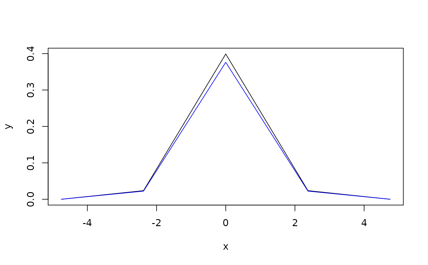
# Manual way with different output structure
df <- meta_x_tbl(form_regrid(d_norm, 5))
## Difference in values due to `form_regrid()` renormalization
plot(enpoint(d_norm, 5), type = "l")
lines(df[["x"]], df[["y"]], col = "blue")