Based on pdqr-function, statistic function, and sample size describe the distribution of sample estimate. This might be useful for statistical inference.
form_estimate(f, stat, sample_size, ..., n_sample = 10000, args_new = list())Arguments
| f | A pdqr-function. |
|---|---|
| stat | Statistic function. Should be able to accept numeric vector of
size |
| sample_size | Size of sample for which distribution of sample estimate is needed. |
| ... | Other arguments for |
| n_sample | Number of elements to generate from distribution of sample estimate. |
| args_new | List of extra arguments for new_*() function to
control |
Value
A pdqr-function of the same class and
type (if not forced otherwise in args_new) as f.
Details
General idea is to create a sample from target distribution by
generating n_sample samples of size sample_size and compute for each of
them its estimate by calling input stat function. If created sample is
logical, boolean pdqr-function (type "discrete" with elements being
exactly 0 and 1) is created with probability of being true estimated as share
of TRUE values (after removing possible NA). If sample is numeric, it is
used as input to new_*() of appropriate class with type equal to type of
f (if not forced otherwise in args_new).
Notes:
This function may be very time consuming for large values of
n_sampleandsample_size, as total ofn_sample*sample_sizenumbers are generated andstatfunction is calledn_sampletimes.Output distribution might have a bias compared to true distribution of sample estimate. One useful technique for bias correction: compute mean value of estimate using big
sample_size(withmean(as_r(f)(sample_size))) and then recenter distribution to actually have that as a mean.
See also
Other form functions:
form_mix(),
form_regrid(),
form_resupport(),
form_retype(),
form_smooth(),
form_tails(),
form_trans()
Examples
# These examples take some time to run, so be cautious
# \donttest{
set.seed(101)
# Type "discrete"
d_dis <- new_d(data.frame(x = 1:4, prob = 1:4 / 10), "discrete")
## Estimate of distribution of mean
form_estimate(d_dis, stat = mean, sample_size = 10)
#> Probability mass function of discrete type
#> Support: [1.8, 4] (23 elements)## To change type of output, supply it in `args_new`
form_estimate(
d_dis, stat = mean, sample_size = 10,
args_new = list(type = "continuous")
)
#> Density function of continuous type
#> Support: ~[1.67226, 4.12774] (511 intervals)
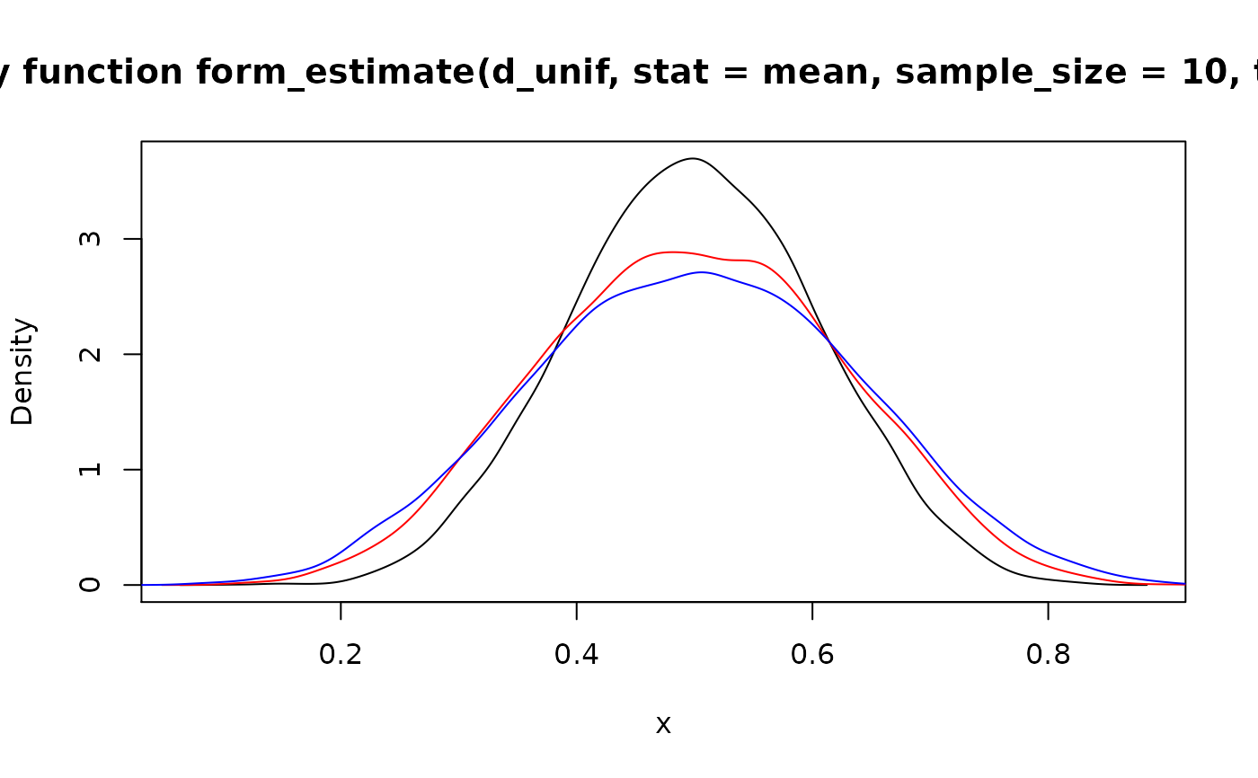
# Type "continuous"
d_unif <- as_d(dunif)
## Supply extra named arguments for `stat` in `...`
plot(form_estimate(d_unif, stat = mean, sample_size = 10, trim = 0.1))
 # Statistic can return single logical value
d_norm <- as_d(dnorm)
all_positive <- function(x) {
all(x > 0)
}
## Probability of being true should be around 0.5^5
form_estimate(d_norm, stat = all_positive, sample_size = 5)
#> Probability mass function of discrete type
#> Support: [0, 1] (2 elements, probability of 1: 0.0318)# }
# Statistic can return single logical value
d_norm <- as_d(dnorm)
all_positive <- function(x) {
all(x > 0)
}
## Probability of being true should be around 0.5^5
form_estimate(d_norm, stat = all_positive, sample_size = 5)
#> Probability mass function of discrete type
#> Support: [0, 1] (2 elements, probability of 1: 0.0318)# }